In my last post I discussed creating Pivot Tables on Mac and PC. Today we will take the next step in Excel,  PivotCharts! Ironically, I find that charts are much easier to work with. But, only if the PivotTable is set up correctly to start with. So, if you missed the creating pivot tables post please watch that video first and then come back and watch today’s video.

Why should I use PivotCharts?

• Flexibility
• Filtering inside the chart
• Formatting

The best reason, in my opinion, to use a PivotChart is the filtering. It basically gives you dynamic chart options with minimal work. Below you can watch my video on how to create PivotCharts or I have a breakdown of the steps you need to take and I have included screenshots.

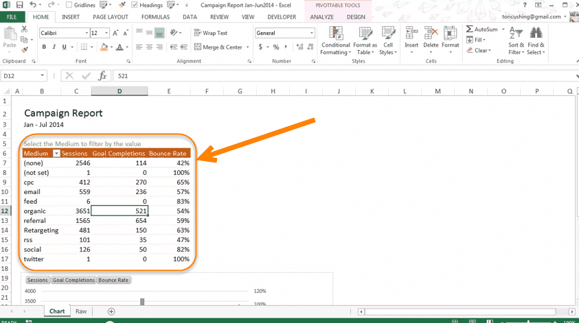
Step 1: Create PivotTable

Reference Excel 104: PivotTables if you need a refresher. But it should be set up something like this.

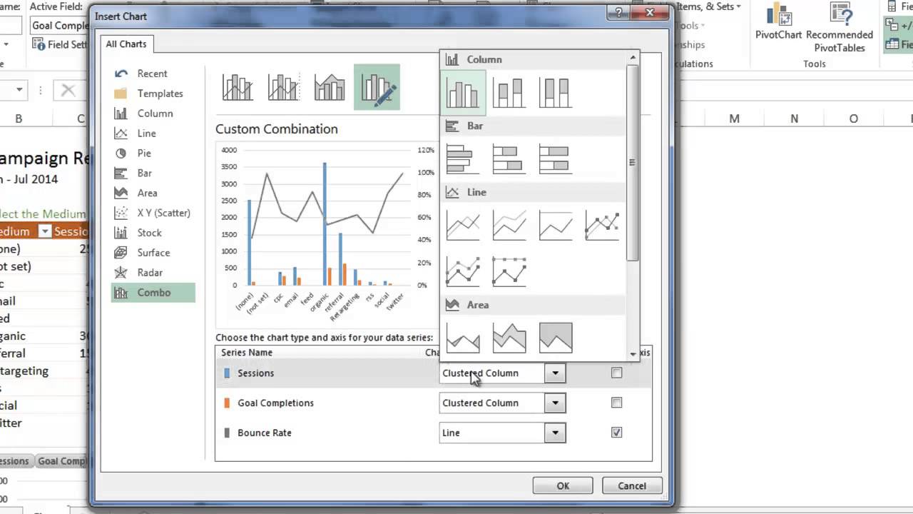
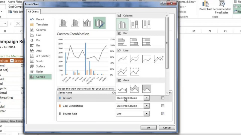
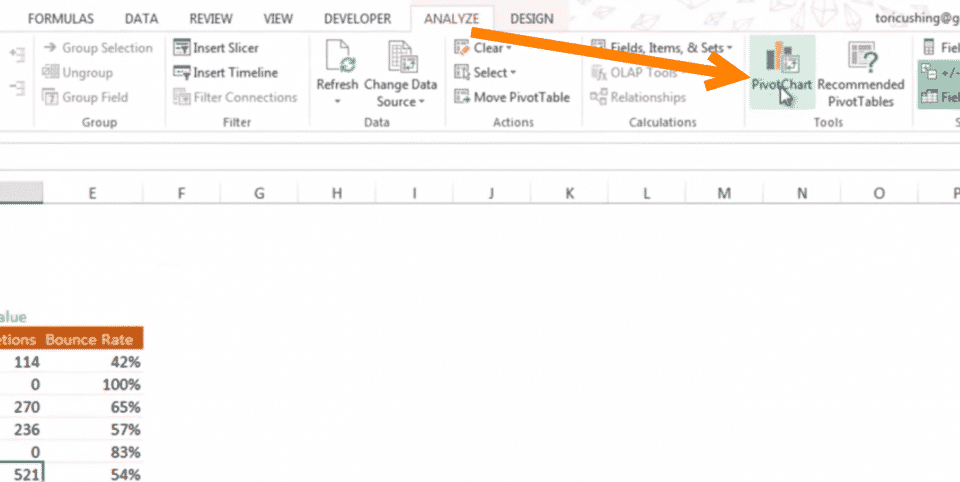
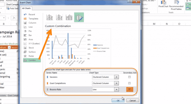
Step 2: Select which type of PivotChart

Here I selected a combo chart to show the session and goal completions on in the column graph.

Step 3: Move data around

I moved the bounce rate onto its own (secondary) axis.

Step 4: Format

You have all the same formatting options in PivotCharts that you have with regular charts. It’s best to make it a client’s business colors.

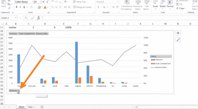
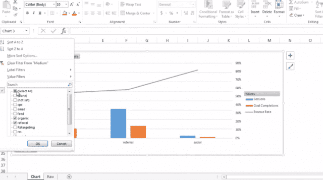
Step 5: Filter

Now that you have your chart all set up, you can filter by your medium values/metric.