At the end of this tuTORIal you will know how to export Screaming Frog data, Google Analytics data, and then bring them together based on whichever value you choose. I will be covering:
- VLOOKUPs
- Basic Formatting
- Conditional Formatting
- Find and Replace tool
- Navigating in Google Analytics
- Navigating in Screaming Frog
Check out part 1 of this series.

Many Internet Marketers have heard of Annie Cushing’s amazing Site Audit Checklist. (If you haven’t checked it out yet, you should.) One of the many tips she released was to make sure that your landing pages are no more than three clicks from the homepage. This level metric is one of the data points we will be pulling in from Screaming Frog, along with Status Codes.
Here is the first part of the video tutorial walk-through. I broke this up into two sections to make it easier for people who have skills in one department over the other. It covers how to export the data you need from Screaming Frog and Google Analytics.
Here is the flip book version!
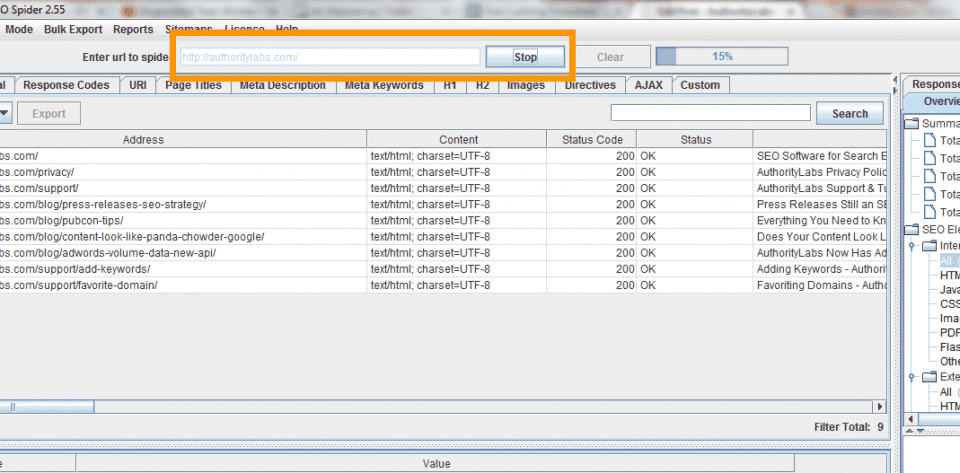
Step 1 – Enter in the site address you would like to analyze and click start.
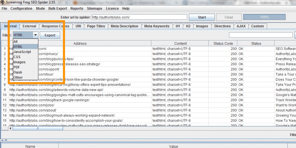
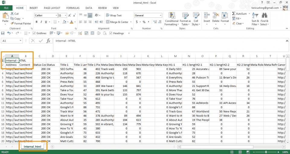
Step 2 – Once the report has finished, export the internal tab by selecting the HTML option and then clicking export.
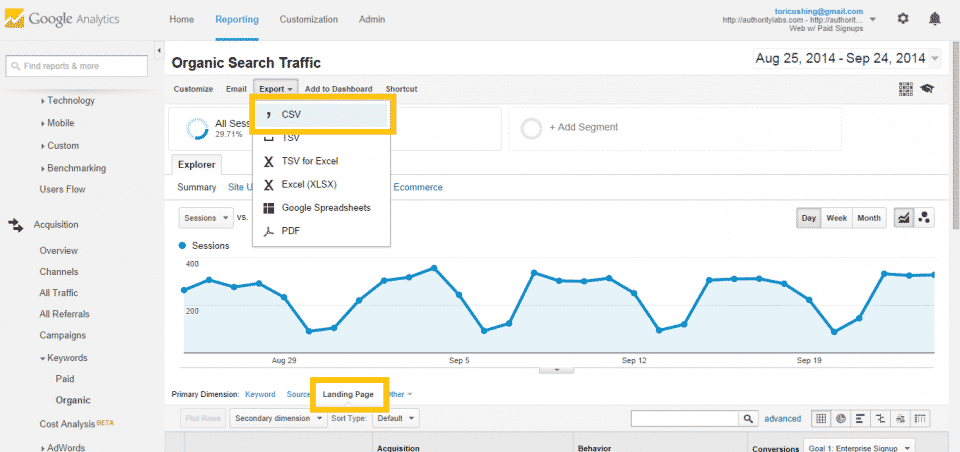
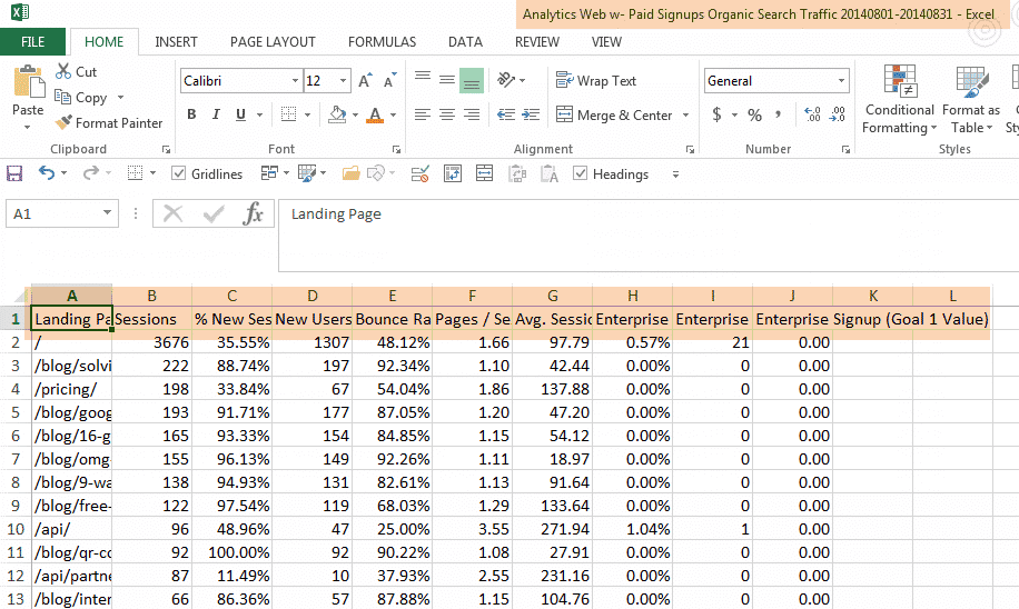
Step 3 – Export the Organic landing pages from Google Analytics. To do this, navigate to Acquisition > Keywords > Organic > Landing Page. Change the rows option to include all of your rows and then select csv export.
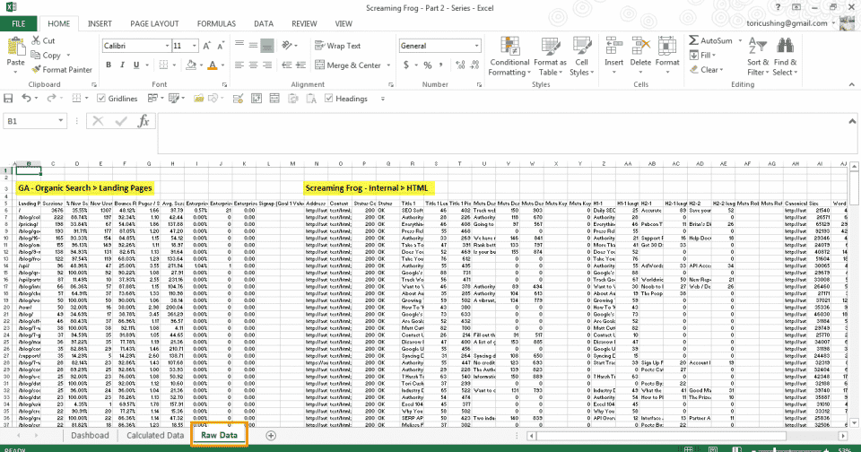
Step 4 – Copy the Google Analytics data and paste it into a Raw Data tab on your dashboard document.
Step 5 – Do the same with the Screaming Frog data.
Step 6 – With all the data together, leave the Raw Data tab untouched from formatting or formulas. Next, bring over the data you would like to have in your dashboard.
Screaming Frog: Address, Level, Status Code
GA: Landing Page, Sessions, % New Sessions, Bounce Rate, Avg. Session Duration
Part 2 – Formatting and Formulas
Step 7 – First and foremost, turn off those gridlines! I know, I’m a broken record.
After pulling in the data to the Calculated Data tab, separate them into two tables. In the first data set (GA), add in two columns one for each of the Vlookup formulas.
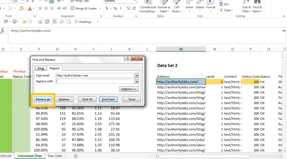
Next, you’ll need to Find and Replace the https://www.authoritylabs.com to switch the Screaming Frog export’s URLs to URIs. To do this, press CTRL + F and select the Replace tab.
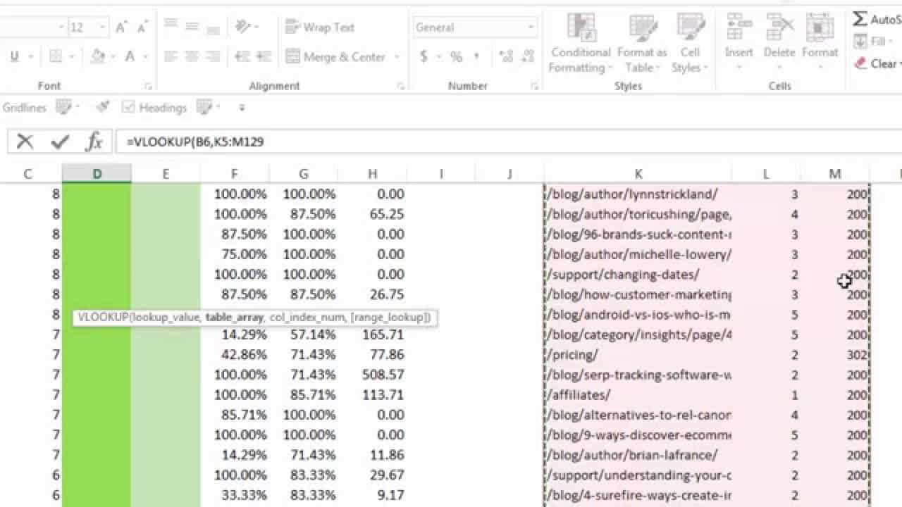
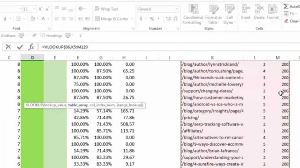
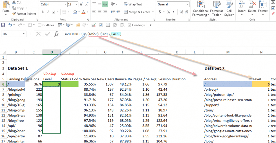
Step 8 – Now you’re ready to write your Vlookup.
- 1st: Select the value you would like to look for. In this case, it’s the homepage or the URI “/”.
- 2nd: Select the range of cells you would like to look for this value in. That would be the Data Set 2 table. Lock down those values by selecting M5:U129 and pressing F4.
- 3rd: Select the column that has the value you would like to retrieve. (In this case it’s the second column.)
- 4th: Type in the word FALSE which means that you want an exact match.
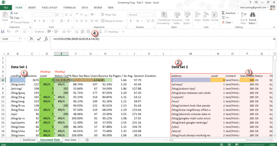
Step 9 – Repeat the process for the Status Code column. Remember to switch the column number to 4.
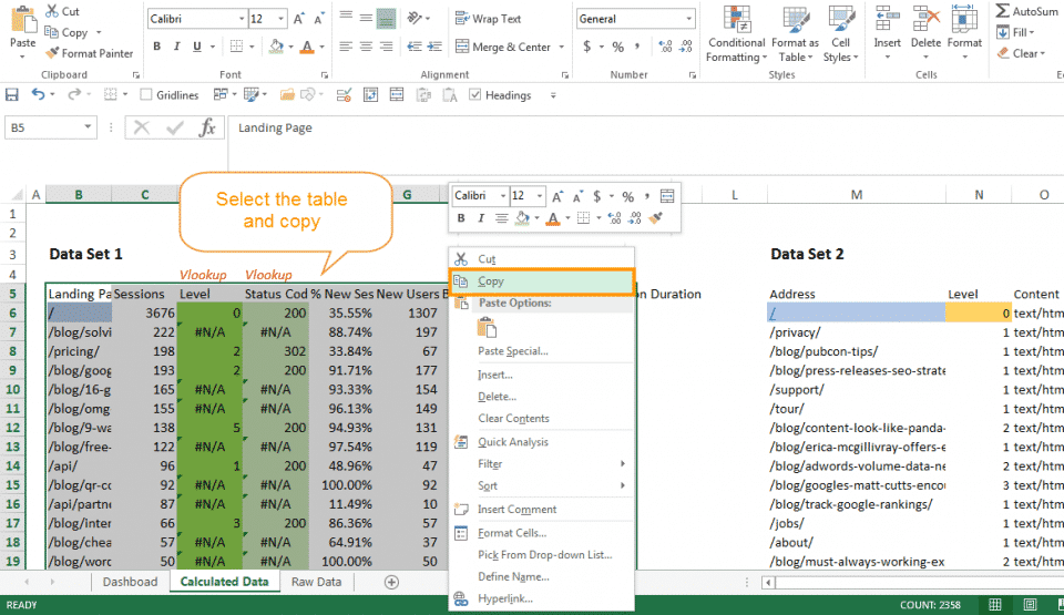
Step 10 – Now that you’ve pulled over the data you want. Select the first data set and bring it over to the Dashboard tab. To do this without messing up your formula values, copy and paste special > values only.
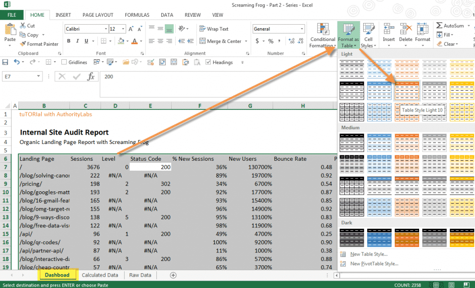
Step 12 – Select the data set and format as a table to get the filtering options.
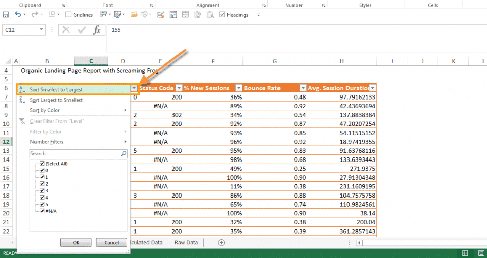
Step 13 – Then filter the levels from smallest to largest. This will put all the “N/A” values at the end of the table.
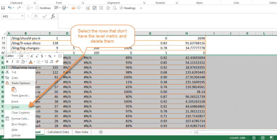
Step 14 – Delete or Hide the rows that don’t have values.
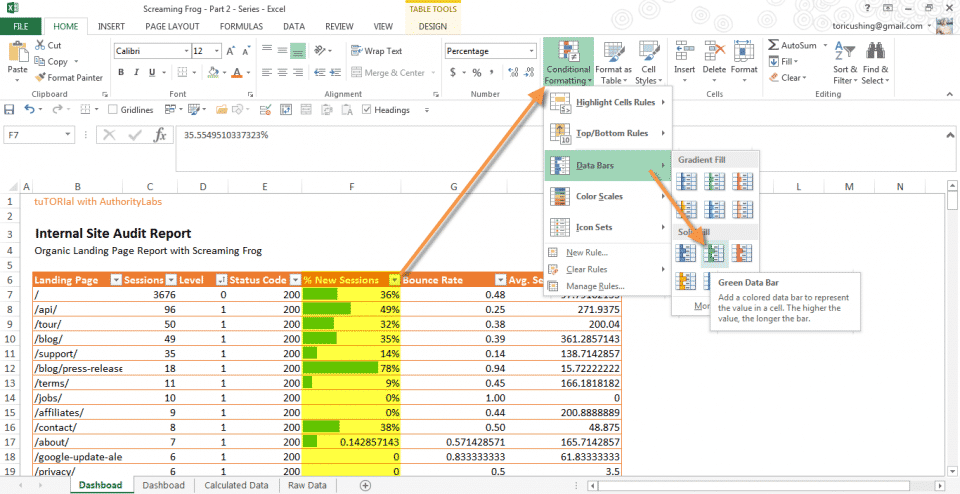
Step 15 – Select the New Sessions column and under the Home tab select Conditional Formatting > Data bars.
Continue to do this with different colored bars for Sessions, Bounce Rate, and Avg. Session Duration.
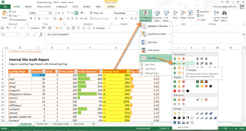
Step 16 – You can do basically the same thing for bounce rate, but instead select the icon set.
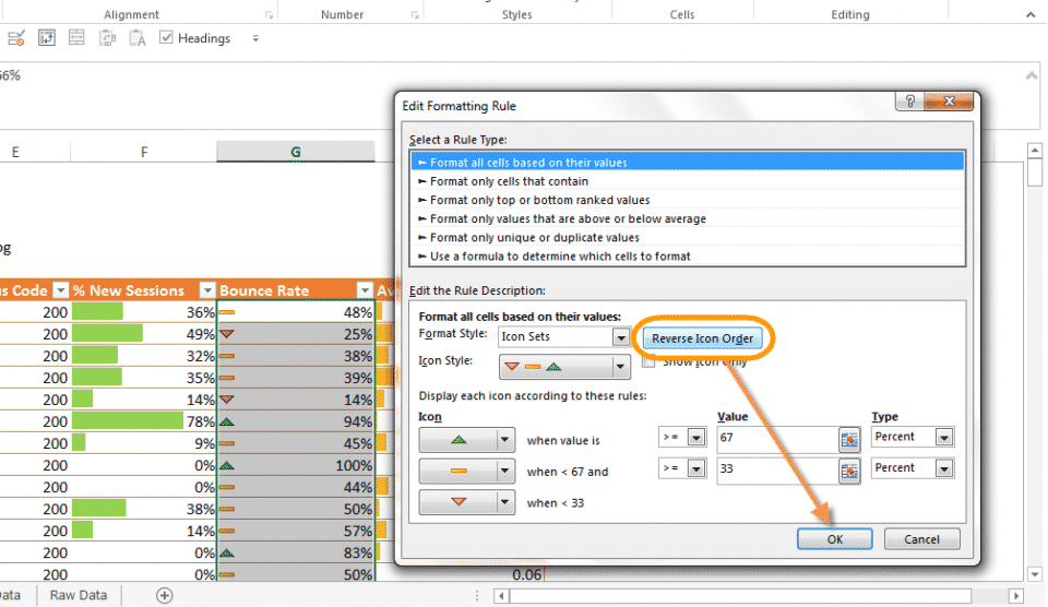
Step 17 – Only one problem. Bounce rate has opposite values as positive. So you will need to switch the positives to negatives. Luckily, Excel gives an easy fix to this. Manage Rules > Double-click on the Icon Set > Reverse Icon Order > Okay.
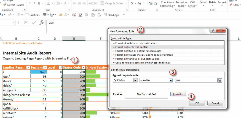
Step 18 – To add in a custom format for scratch, select the column > Conditional Formatting > New Rule > Format only cells that contain.
From there select a cell value that is equal to = 200. 200 is a good status code, so I format it as blue.
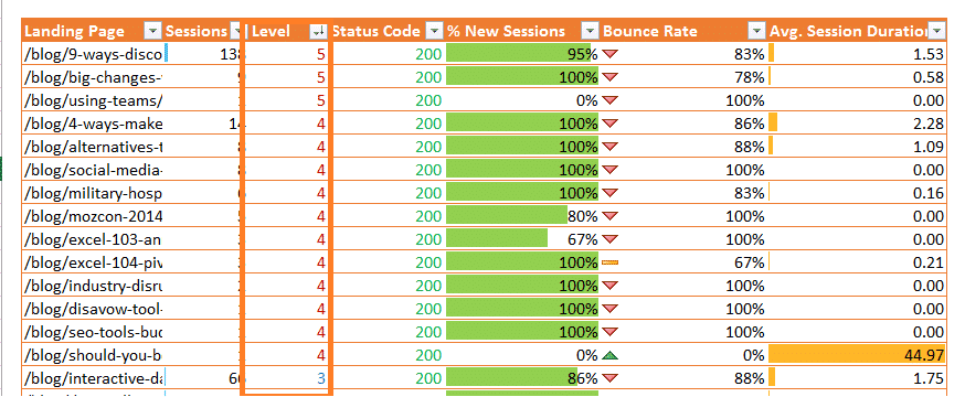
Step 19 – You can do the same thing for the Level metric and set the values that were greater than 3 to red.
Step 20 – Now you’re finished! Go forth and make your own awesome report!